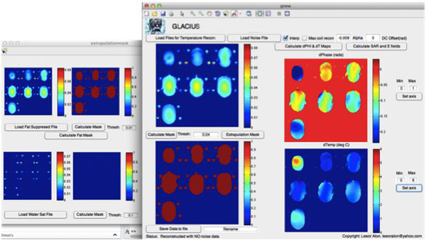
We are sharing software for rapid and optimal reconstruction of temperature maps from raw Siemens MRI data.
GLACIUS provides robust reconstruction of phase information from two- and three-dimensional gradient echo acquisitions with multiple receive coils. A Windows version of the software is also available.

Optimal Phase Reconstruction for Thermometry
The difference of two phase maps—one acquired before RF heating, the other afterward—yields a map of magnitudes proportional to the change in temperature. Assuming that Z1 is the complex image of the pre-heating acquisition and Z2 the complex image of post-heating acquisition, we can calculate the angle between the phases, and the change in phase between the images is
where Im( ) and Re( ) are imaginary and real number operators, respectively.
Since the complex conjugate and the inverse of the complex conjugate of Z2 have the same phase, the above equation can be rewritten as
(The four-quadrant function, known as ATAN2 in MATLAB, is preferable to the tan-1 function.)
Many MRI coils have more than one element. GLACIUS uses the following algorithm
Reference
Reconstructions of phase contrast, phased array multicoil data.
Magn Reson Med. 1994 Sep;32(3):330-4. doi: 10.1002/mrm.1910320308
Get the Code
The software available on this page is provided free of charge and comes without any warranty. CAI²R and NYU Grossman School of Medicine do not take any liability for problems or damage of any kind resulting from the use of the files provided. Operation of the software is solely at the user’s own risk. The software developments provided are not medical products and must not be used for making diagnostic decisions.
The software is provided for non-commercial, academic use only. Usage or distribution of the software for commercial purpose is prohibited. All rights belong to the author (Leeor Alon) and NYU Grossman School of Medicine. If you use the software for academic work, please give credit to the author in publications and cite the related publications.
How to Use
Click on “Load Files for Temperature Recon” and select your pre- and post-heating sequences. Once the files are selected, a note in the bottom-right corner will read “processing.” Once the files are loaded, the note will read “Great success.”
Enter the mask threshold—typically a number between 0.01 and 0.2—and press “calculate mask” button.
Adjust the proton resonance frequency shift coefficient to the desired number—typically 0.01±0.002 ppm/ºC.
Click “calculate dPHI & dT Maps” button.
Once the phase maps and dT maps are calculated you can adjust the threshold of the maps by choosing a minimum and maximum values and clicking “set axis” button.
Oil Phantoms and B0 Offset Correction
In temperature mapping experiments, oil phantoms are added to the setup to account for B0 changes that are not temperature related. Click on the ”data cursor” icon in the upper area of the window and click on the region where the oil phantoms are located in the phase map. When you hover the pointer over the oil phantom, the software will display a phase value in radians.
To correct any DC B0 offsets that might occur in the MR system, use the DC box in the top left area, and enter the magnitude of the observed offset but with the opposite sign. For example, if a -0.05 radian is observed when putting the cursor on the phase map, then add 0.05 to the DC offset field.
Click “calculate dPHI & dT Maps” to compute the temperature difference.
If the correction is sufficient, you can save the file by entering a filename in the bottom left corner and clicking “save.”
If the correction is not sufficient, click on “extrapolation mask.” This will open a new window that fits a polynomial to estimate a B0 map in two- or three-dimensions, based on the phase measured in the oil phantoms. In the new “extrapolationmask” window, click “load water sat file” and chose a water suppression image to be loaded.
Once the mask has loaded, enter the threshold for the new oil mask and click “calculate.” Then, choose the polynomial order. The program supports polynomial orders of 1 through 4. The default is two dimensions. If you want the polynomial to be conducted in three dimensions, check the “3D” checkbox. Click “calculate extrapolated field” and wait until the extrapolated B0 is shown.
Then, go back to the main window and check the “interp” checkbox in the center-top area. Set DC offset to 0 and click “calculate dPHI & dT Maps.”
You may have to play with the oil phantom mask, polynomial order and 2D/3D features to fine-tune the fits. Once the fits are calibrated, save the file. In the saved MATLAB file, “handles.dT” corresponds to the temperature difference variable computed by the program.
Contact
Questions about this resource may be directed to Leeor Alon, PhD.
